

Despite being pretty straightforward concepts to grasp, latency and throughput can become very complex subjects when we dive into them.
Even at a shallow glance, when we are dealing with systems’ design, they can lead to hard situations, and knowing them well can be the difference between a good and a bad architectural decision.
So, without any further delay, let’s get started.
So… what’s latency again?
Latency can be understood as a simple delay between two desired events. These events can be whatever you want to measure, even if it’s not related to computer science, e.g., the time you take to read this article after you’ve decided to do it  .
.
For the sake of contextualization, we’ll refer to latency in this article as being always related to network communications through the Internet.
It’s worth mentioning that we’re affected by latency in everything we do through the Internet, but in some way, we’re used to it. Things get worse when we actually notice this latency.
Two good examples of bad — or perceptible — latency are:
- Lag (well known among our fellow gamers): the perceived time between a command and the consequent action being taken on the screen.
- Space communication: the waiting time between the instant a message or command is sent and the instant it is received by the counterpart when communicating with our satellites, rovers, etc.
“It generally takes about 5 to 20 minutes for a radio signal to travel the distance between Mars and Earth, depending on planet positions.”
But don’t worry, we’ll discuss more of this concept later on.
… and throughput?
Well, the throughput concept is even more straightforward than latency: it’s the amount of data — or something else — that can be transferred within a specific period.
Again, this concept is not exclusive to computer science, but when it comes to the context of this article, it will always be related to network communications.
Some examples of throughput can include:
- A user network of 100 Mbps
- An internal server or data center network of 5 Gbps
Once more, the throughput, just as latency, can be affected by several external factors. In this case, the physical medium is usually the limiting factor that works against you.
Last but not least: Round-trip delay
Also known as round-trip time or RTT, it’s the measured delay for a network request to reach the destination host and go back — usually in the form of a response to the request.
In a stable network, the RTT will be roughly double the common latency. But it can vary a lot depending on the network condition.
Let’s design a system! Yay!
Now that these concepts are fresh in our minds, let’s start using them in a real-life problem that many of you could have already faced or will face someday: store and transfer large files over the Internet.
Imagine you have to store several big files — that can reach even more than 10 GB — and your end-users will have to download these files frequently.
As you might have noticed, this is only a part of a bigger system. But it’s enough to visualize the important concepts we need. You can assume the other parts are already defined and running smoothly.
A naive solution
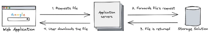
A simple way to start is spinning up a bunch of servers to deal with the users’ requests which will be responsible to give them the file they want to download. Once we have our application servers in place, we have to link them with our files’ source.
The files will be stored in a centralized storage solution provided by our cloud provider and easily accessible by our application servers.
This seems to solve our problem, at least partially. A requirement that wasn’t mentioned is that our solution is global and will be accessible for users spread throughout the whole world. This is something we should take into account when designing our system.
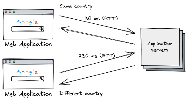
With our previous knowledge about latency, it isn’t hard to figure out that users from different regions will suffer different — and high — latencies accessing our servers.
Measuring these latencies, we can see a big difference between users from different countries. The geographically closer the user is to the servers, the lower their latencies will be.
This is caused by the limits of the physical medium: unlike your in-house wi-fi, the Internet needs cables to transmit data throughout the world and the signal is limited to the speed of light — which is very fast, but not infinite. The more distant the sender is from the receiver, the longer it will take to deliver a message — the latency will be higher.
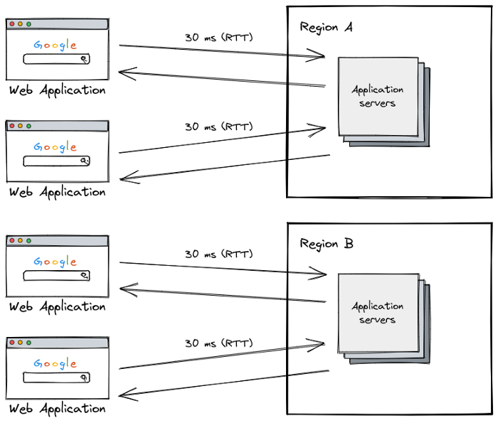
Well, there aren’t many things we can do other than bring the servers closer to the user, that is, we’re willing to pay a bit more to use the regions provided by our cloud provider to distribute our application servers among them, reducing the latency for everyone.
Everything seems to be fine now. Our users aren’t suffering from high latencies anymore. At least not from the application servers’ point of view.
And what about the communication between our application servers and our storage solution? Is it optimized?
Well, maybe we were too naive: issues with our first attempt
Despite the communication between the users and the application servers being well addressed now, our storage solution is a little overlooked. Some users are still facing issues — slowness, so to speak — when downloading files. But why?
You probably remember that our design utilized a centralized storage solution. Since you think like an engineer, you probably have already thought that this is the issue here. We should break down our monolithic storage solution into several regions!
Well, probably you are right, but why should we do that? Let’s take a closer look.
Latency vs. throughput
Our application servers are hosted on a decent cloud provider with an excellent network throughput of roughly 5 Gbps. Our users are downloading 10 GB files within a private network of roughly 100 Mbps.
Considering our servers’ network isn’t at full load, shouldn’t the users be able to download files at their networks’ maximum speed?
It’s important to notice here that 100 Mbps is the throughput of the users’ network, and it doesn’t depend on the users’ latency. Latency and throughput are different concepts.
In a 100 Mbps network, users can transfer data at a maximum speed of 12.5 MB/s. That is, the file will take 819.2 seconds to finish downloading — something between 13 and 14 minutes.
100 Mbps / 8 bits (1 byte) = 12.5 MB/s10240 MB / 12.5 MB/s = 819.2 s
If we take into account the latencies involved in the process of starting the download, that’s the scenario we see:
User 1 — in the same region as the storage servers — roughly 30 ms of communication overhead.
7 ms for the file request to reach one of the application servers
8 ms for the application server to forward the request to the actual storage server
8 ms for the storage server to respond to the application server
7 ms for the application server to respond to the user
User 2 — in a different region than the storage servers — roughly 230 ms of communication overhead.
15 ms for the file request to reach one of the application servers
100 ms for the application server to forward the request to the actual storage server
100 ms for the storage server to respond to the application server
15 ms for the application server to respond to the user
As we can see, storage servers being far from part of the application servers indeed causes some increased latencies. But the difference is very small — something around 200 ms — compared with the total lead time of 14 minutes to complete the download.
But the fact that some users are facing slowness is still a reality. Perhaps we’re missing something here.
The TCP protocol
You may have heard about the sliding window algorithm used by the TCP protocol to achieve flow control over the transmission of the packets. If you haven’t, don’t worry, we will explain it briefly here.
The sliding window is the way the TCP protocol limits the number of packets to be sent until the sender gets acknowledgment that they have been received. This mechanism prevents the sender from wasting bandwidth in the situation that the packets aren’t being delivered successfully.
As you can see in the figure below, packets enumerated from 5 to 10 are in the sending window, which means these 6 packets were sent to the receiver and the sender is waiting for the acknowledge signal for each packet.
This signal indicates the packet was received successfully and can be removed from the sender’s buffer.
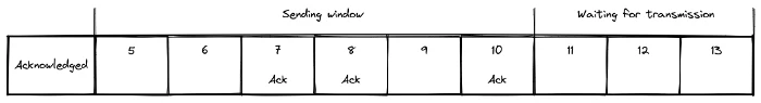
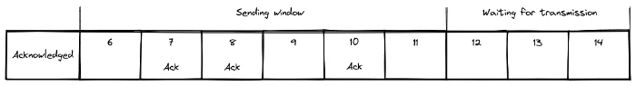
When the sender receives the acknowledge signal referring to packet number 5, the window is shifted to the right, allowing packet 11 to be sent.
The TCP protocol makes use of this concept of the sliding window to obtain several benefits, among them:
-
Avoid flooding the network if the receiver is not able to process more packets
-
Taking on the transmission mechanism, making it possible to know if any packet was lost and then retransmitting it
So, what does this whole thing have to do with our slowness issue? May you ask.
Everything! As you could have already noticed, any packet loss on this transmission mechanism will require retransmission to happen, which will take the whole TCP round-trip delay to deliver it and, since the TCP protocol doesn’t send more packets while the sliding window isn’t shifted, our end-users will notice a slowness with their downloads.
The bigger the round-trip delay, the slower the download. Isn’t it funny how two completely different concepts start to work together to make our life more difficult?
Well, this is our job, after all. Damn TCP!
In fact, there is an equation (Mathis et al) that can be used to estimate the real network throughput based on the packet loss rate.
I won’t add this equation here for simplicity matters. For more information, you can reach out to the original article here.
But there is a good simulation tool — based on the same equation — that we can use to have at least a glance at the effect that high latencies can cause on our network throughput.
For the next simulations, we’ll keep the link bandwidth fixed at 100 Mbps and the file size fixed at 10 GB. Our packet loss rate is 0.0001%.
For the first simulation, we’re using a round-trip delay of 30 ms.
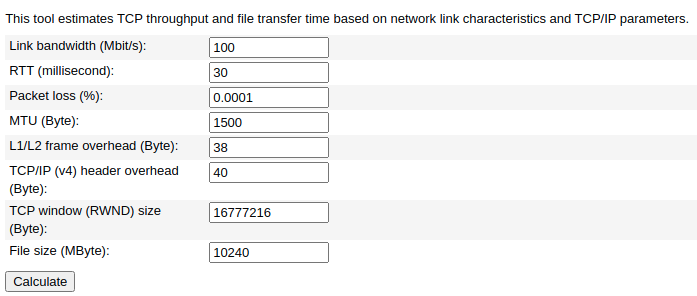
As a result of this simulation:
Expected maximum TCP throughput (Mbit/s): 94.9285Minimum transfer time for a 10240 MByte file (d:h:m:s): 0:00:14:23
It means that our 100 Mbps theoretical network throughput is reaching, at maximum, 95 Mbps due to the packet losses and retransmission.
For our second simulation, we’ll use a round-trip delay of 230 ms.
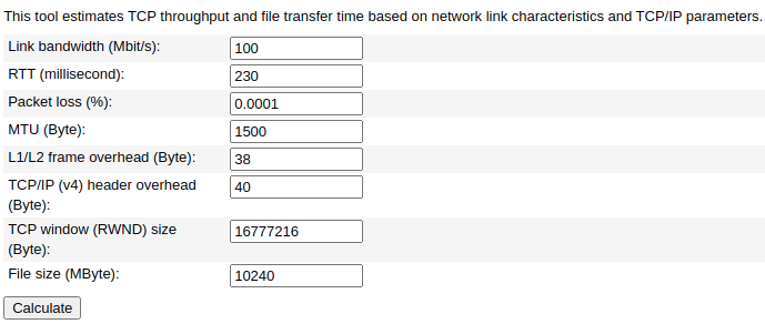
As a result of this simulation:
Expected maximum TCP throughput (Mbit/s): 50.782609Minimum transfer time for a 10240 MByte file (d:h:m:s): 0:00:26:53
As you can see, the difference is huge! Our download lead time almost doubled, and our users’ networks are being underutilized — almost half of the full capacity. Now that we know what’s happening, let’s fix it.
Fixing our design
How can we improve the network throughput in this case? There are, actually, a few alternatives, as follows:
-
Increase TCP’s window
-
Decrease the packet loss rate
-
Decrease the round-trip delay
The first option isn’t actually very helpful in most cases. Increasing the TCP’s window will only help if we are in one of the two situations:
-
The servers are configured to use a small sending window — which isn’t our case.
-
The users are configured to use a small receiving window — this is also not the case. As you can see in the simulation figures, the RWND parameter is something around 16 MB.
Even if the users’ receiving window was small, we couldn’t configure each user’s machine to increase it. Definitely, that is not an option for us.
It’s also worth mentioning that the TCP protocol itself has a mechanism to negotiate window sizes between the parts. The configuration mentioned here limits only the maximum size these windows can reach.
The second option is to decrease the packet loss rate in our users’ network. But our servers are already hosted in a decent cloud provider and we don’t have control over the network between the users and our servers — this is the whole Internet!
We’re left with the third option, reducing the round-trip delay between the users and our storage servers. As you may have guessed at this point, this is where regions for our storage solution come in handy.
We can replicate the storage solution for each region we have application servers running, drastically reducing the latency between them. Of course, we’ll have some extra concerns regarding the replication mechanism and all the stuff that comes together, but we’ll not worry about that now.
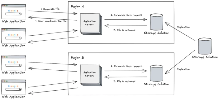
Now the end-users can use their networks at almost full load, and they’re not experiencing slowness anymore.
With that, we were given an extra gift that you may haven’t noticed yet. We have redundancy for our storage solution, which means our availability is better than before, moving us towards a highly available system.
But that’s a subject for another day.
Conclusion
Even when dealing with straightforward concepts, we should take extra care to understand the real issues behind the scenes.
Even though latency and throughput are different concepts, we can face some situations where they have a direct impact on each other — like the example we saw here.
Knowing both of them is crucial to better address the issues we may face while designing our systems.
It’s also important to evaluate the pros and cons of each possible solution we have available.
References
The Macroscopic Behavior of the TCP Congestion Avoidance Algorithm (Mathis et al)
